mSWE-GNN: paper walkthrough + pretrained-model reproduction — FAST VARIANT (Multi-scale hydraulic graph neural networks for flood modelling)¶

Paper: Bentivoglio, Isufi, Jonkman & Taormina, Multi-scale hydraulic graph neural networks for flood modelling, Nat. Hazards Earth Syst. Sci. 25, 335–351, 2025, doi:10.5194/nhess-25-335-2025 (open access, CC BY 4.0). Code: mSWE-GNN-main/ (upstream repo v1.1, Nov 2024, git 529bb92). This notebook lives in the repo root and imports the authors' own utils/, models/ and training/ modules. Data: Zenodo 10.5281/zenodo.13326595, unpacked into database/raw_datasets_mesh/ (100 D-HYDRO simulations) and database/raw_datasets_dk15/ (11 dike-ring-15 simulations), then converted into database/datasets/{train,test}/*.pkl.

What this notebook does¶

Two layers of content, interleaved and ordered the way the paper is written:

1. Paper walkthrough (markdown + the paper's own figures, taken from the open-access article page and stored in paper_figures/): the research problem and the gap, the method (multi-scale mesh, architecture, boundary conditions, loss), the experimental setup, the results, the discussion.
2. Reproduction (code cells, already executed on 1×H100 with outputs saved): training is completely frozen. We only load the 17 checkpoints shipped with the repo (results/Pareto_front/models/K{2..5}_F{16,32,50,64}.h5, results/finetuned_dk15.h5), roll them out on the real test sets and visualise the result. Subsections titled "In the code / data" are the reproduction; everything else is the paper.

Environment: Python 3.10 or 3.11 with torch 2.1.0, torch_geometric 2.4.0 and lightning 2.0.9.post0 — environment-cpu.yml and requirements-cpu.txt pin the exact set, and §0.0 below has the build, data and runtime steps for the I-GUIDE Platform, including why conda cannot be used there.

Fast variant — read this first¶

This is the executable version of the walkthrough, trimmed so it finishes in roughly 8 minutes on a CPU-only JupyterHub container instead of about 4 hours. Three changes, each marked FAST VARIANT in the code with the original line left commented above it:

Change	Full notebook	Here	Saves
Synthetic test simulations	20	3	~11 min
16-checkpoint Pareto sweep	run	skipped, plotted from the authors' csv	~3.5 h
Dike-ring-15 test simulations	10	2	~11 min

The metrics printed here are computed over 3 simulations, not 20, so they will not match the paper or the full notebook. They are for checking that the workflow runs, not for quoting. For the reproduction numbers — CSI₀.₀₅ 0.803 against the authors' recorded 0.830, and the depth MAE that does — see test_pretrained_EN.ipynb, which carries the saved outputs of a full 20-simulation run on an H100 and needs no execution to read.

Nothing else differs: the same checkpoints, the same data pipeline, the same autoregressive rollout, the same metric definitions and the same figures.

About the saved outputs below. They come from one execution on a single H100, so the timings and speed-up figures in them are GPU figures. On the CPU-only container this variant targets, expect roughly 40 s per synthetic simulation and 90 s per dike-ring-15 simulation — about 8 minutes end to end, against a few seconds here. The accuracy numbers are hardware-independent; only the timings are not. Re-run the notebook and your own outputs replace these.

0.0 Before you run this¶

Every output below is already saved, so this notebook can be read end to end without running anything, without an environment and without the data. The steps here are only needed to re-execute it.

1. The kernel¶

Pick Python (mswegnn) from the kernel menu. If it is not listed, build it from a Terminal:

bash setup_iguide_kernel.sh

That script uses python -m venv and pip rather than conda, on purpose. On this hub conda env create is killed by the out-of-memory killer while parsing conda-forge repodata and reports only Killed: the container is capped at 8 GiB and conda's classic solver exceeds it. pip needs a fraction of that memory. Disk is not the constraint here — home is measured in terabytes.

None of the roughly 26 kernels already installed on the hub will do. The closest, geoai, has PyTorch 2.4.0 but no torch_geometric, and lightning must be exactly 2.0.9.post0, because the upstream code calls load_from_checkpoint on an instance, which 2.1 and later reject with a TypeError.

2. The data¶

The 3.1 GB of preprocessed pickles are not in the repository. Rebuild them from Zenodo:

wget -c -O database/raw_datasets_mesh.zip "https://zenodo.org/records/13326595/files/raw_datasets_mesh.zip?download=1"
wget -c -O database/raw_datasets_dk15.zip "https://zenodo.org/records/13326595/files/raw_datasets_dk15.zip?download=1"
python -c "import zipfile; [zipfile.ZipFile(f'database/raw_datasets_{n}.zip').extractall('database') for n in ('mesh','dk15')]"
python scripts/build_real_pickles.py

unzip is not installed on this hub, hence the Python one-liner. Zenodo sometimes answers 502 or 504 on the dike-ring-15 archive; wget -c resumes where it stopped. The build takes about 13 minutes.

The training split is required even though nothing is trained here: the feature scalers are fitted on it. A test-only download will not work.

3. What it will cost¶

Measured at roughly 40 s per synthetic simulation and 90 s per dike-ring-15 simulation on a CPU container, against 0.19 s and 1.5 s on an H100:

4. Did it work?¶

These are 3-simulation figures. The 20-simulation values, which are the ones comparable to the paper, are in test_pretrained_EN.ipynb.

Two structural checks that do not depend on hardware: the load should report train 60 / val 20 / test 20 simulations, and test simulation 0 should have 11 837 / 2 961 / 741 / 186 cells across the four scales. Those came out identical on two unrelated clusters, so they are a good signal that the data pipeline rebuilt correctly.

0. Reproduction setup: environment, data and checkpoints¶

0.1 Data and checkpoint check¶

config.yaml is the authors' reference configuration; its saved_model field points at the checkpoint to be tested. create_model_dataset loads both the train and the test pickle (the training split is used only to fit the feature-normalisation scalers — no training happens here).

0.2 Load the test dataset (20 synthetic simulations)¶

Each sample is a PyG Data object: WD/VX/VY have shape [num_nodes, 97] (96 h, one frame per hour; the config's temporal_res=120 min subsamples every other frame into 49 steps); node_ptr delimits the node ranges of the 4 scales; BC is the inflow hydrograph.

1. Introduction: the problem and the gap¶

The problem. Dike- and dam-breach flood mapping relies on numerical models that solve the 2-D shallow water equations (SWE), such as D-HYDRO / Delft3D FM. They are accurate, but one 96-hour simulation takes hours (12 h 20 min for the 20 synthetic cases and 47 h 15 min for the 10 dike-ring-15 cases, see Table A1), which rules out probabilistic, many-scenario assessment. Deep-learning surrogates can be orders of magnitude faster, but most of them have to be retrained for every new area.

The starting point. The authors' earlier SWE-GNN (a hydraulic-based graph neural network) treats the finite-volume mesh as a graph and lets a GNN propagate water between neighbouring cells. It transfers to unseen domains and can embed physical constraints.

The gap (the four limitations listed in the abstract):

1. It cannot represent large differences in propagation speed — information travels one hop per layer, so a fast flood wave needs many layers.
2. Training becomes unstable with many layers — SWE-GNN needs 10–18 of them (Table D1); deep message passing is hard to train and slow at inference.
3. It cannot take time-varying boundary conditions, such as a breach discharge hydrograph.
4. It needs initial conditions from a numerical solver.

The proposal: mSWE-GNN (multi-scale SWE-GNN)

• Build several mesh resolutions over the same domain (4 scales) and arrange them into a U-shaped multi-scale GNN: fine → coarse → fine. One hop on a coarse scale covers a long physical distance, so a few layers per scale (2–5) let information cross the domain, while the finest scale (which holds most of the nodes) does less work than before.
• Inject the time-varying discharge hydrograph through a ghost cell as a directed edge, and roll out autoregressively from a dry bed ($t=0$, no water), with no dependence on a numerical solver.
• Use only rotation-invariant inputs (area, elevation, roughness, water depth, magnitude of unit discharge, dual edge length).
• The decoder is a 1-D convolution along the time axis plus an MLP that outputs the next $h$ and $|q|$ directly, with a ReLU enforcing non-negativity.

Headline results (from the abstract): MAE ≈ 0.05 m for water depth and ≈ 0.003 m² s⁻¹ for unit discharge on the synthetic test set; speed-up > 700× on the real case study (dike ring 15 in the Netherlands), reaching CSI$_{0.05\,\mathrm{m}}$ = 87.68 % after fine-tuning on a single simulation.

2. Methodology¶

2.0 Overall framework (paper Fig. 1)¶

Fig. 1 — The model $\Phi(\cdot)$ takes (blue box) a fine mesh and its progressively coarsened versions $\mathcal{M}_{1..M}$, the static inputs $\mathbf{X}_s$ defined on them (DEM and so on), the dynamic inputs $\mathbf{U}^{t-p:t}$ (water depth and discharge at the previous $p+1$ times) and the boundary condition (the current slice of the breach hydrograph); it outputs (orange box) the hydraulic variables at the next time, $\hat{\mathbf{U}}^{t+1}$. Feeding the output back in as the next input rolls the prediction forward to $T$. The lower half is the multi-scale module: a GNN runs on the fine scale (purple arrows), the state is downsampled (green) to the coarser scale for another GNN, and after the coarsest scale it is upsampled step by step (yellow-green) and added to the matching downward features (red skip connections), before the decoder produces the output.

Figure source: Bentivoglio et al., NHESS 25, 335–351, 2025, doi:10.5194/nhess-25-335-2025, CC BY 4.0.

2.1 Multi-scale mesh and multi-scale graph (§2.1, paper Fig. 2)¶

Mesh generation (only the boundary polygon of the area is needed): MeshKernel first produces a coarse mesh; splitting every edge in two and connecting the new points gives the next finer level; the result is then orthogonalised (required by Delft3D's staggered grid) and over-elongated cells are removed, leaving a mixture of triangles and quadrilaterals. Repeating this yields $M$ scales (4 in this paper).

Graph definition: nodes are cell barycentres, edges connect cells that share a face (the dual graph). The rule for connecting scales is simple: if a fine cell's centre falls inside a coarse cell, a directed inter-scale edge is added between the two.

Fig. 2 — (a) A three-scale multi-scale graph can be written as one block adjacency matrix: the diagonal blocks $\mathbf{A}^m \in \mathbb{R}^{N^m\times N^m}$ are each scale's own adjacency matrix, and the off-diagonal blocks $\mathbf{P}^{m\to n} \in \mathbb{R}^{N^m\times N^n}$ ($n = m\pm1$) are the prolongation matrices between neighbouring scales; non-adjacent scales are zero. (b) Example connection between a fine mesh $\mathbf{A}^1$ and a coarse mesh $\mathbf{A}^2$: $\mathbf{P}^{2\to1}$ links one coarse cell to all the fine cells it covers.

Downsampling / upsampling (Eq. 5–6):

• fine → coarse: mean pooling, a coarse node's features are the average of the fine nodes attached to it (no parameters);
• coarse → fine: a learnable operator, $\mathbf{h}^{m}_{d,i} \leftarrow \psi_{m+1\to m}(\cdot)\cdot \mathbf{h}^{m+1}_{d}$, where multiplying by the coarse node's dynamic features guarantees that water only propagates down to the fine cells if the coarse cell holds water.

Figure source: Bentivoglio et al., NHESS 25, 335–351, 2025, doi:10.5194/nhess-25-335-2025, CC BY 4.0.

In the code / data: the four mesh scales of test sim 0¶

Each simulation's domain is a random polygon; meshkernel builds a triangular mesh and refines it three times. The four scales hold roughly 10 000 / 2 500 / 600 / 150 cells. The coarse scales are what let information cross the domain within a few GNN layers (the long-range action of shallow-water waves).

2.2 Architecture: encoder → processor (U-shaped multi-scale GNN) → decoder (§2.2)¶

Encoder (Eq. 2) — three shared three-layer MLPs map the inputs into a latent space of dimension $G$:

• static node features $\mathbf{x}_{s,i} = (a_i, e_i, m_i, w_i)$: cell area, elevation, Manning roughness, (boundary) water level → $\phi_s$;
• dynamic node features $\mathbf{x}^t_{d,i} = (h^{t-p:t}_i, |q|^{t-p:t}_i)$: water depth and unit-discharge magnitude over the previous $p+1$ times ($p=2$; the code's previous_t=3 is the same 3 frames) → $\phi_d$;
• edge features $\boldsymbol{\varepsilon}_{ij} = (l_{ij})$: dual edge length → $\phi_\varepsilon$. Static and dynamic features on the coarse scales come from mean pooling the finest scale.

Processor: the GNN layer (Eq. 3–4)

$\psi:\mathbb{R}^{5G}\to\mathbb{R}^{G}$ is an MLP and $\mathbf{W}\in\mathbb{R}^{G\times G}$ is learnable. The difference term $\mathbf{h}_{d,j}-\mathbf{h}_{d,i}$ models the hydraulic gradient: only a node that already holds water can push water to its neighbours. That is the physical constraint built into the model, and the reason it is called "hydraulic-based".

U-shaped ordering: $L$ GNN layers per scale (K in the code), downsampling fine → coarse and upsampling coarse → fine; after upsampling, the features are added to the downward branch at the same scale (skip connection, Eq. 7: $\mathbf{h}^m_d \leftarrow \mathbf{h}^{m\downarrow}_d + \mathbf{h}^{m\uparrow}_d$) before the next group of GNN layers.

Decoder (Eq. 8)

The first term is a 1-D convolution along the time axis ($\mathbf{w}_p\in\mathbb{R}^{p+1}$ learnable, effectively a linear extrapolation of the last few frames); the second is a three-layer MLP decoding the latent features. The ReLU keeps depths and discharges non-negative. Note that this predicts the absolute value at the next step, not an increment as SWE-GNN does (Table 3 ablates a residual decoder).

The configuration selected in the paper: $L=4$ layers per scale, $G=64$, 4 scales, about 811 000 parameters — that is K4_F64.h5 in the repo, loaded in section 3.4 below. Architecture.png in the repo root is a high-resolution diagram of the same architecture.

2.2.1 Receptive field and compute cost: why "4 layers per scale" is enough¶

The sentence above — "the coarse scales let information cross the domain within a few GNN layers" — needs to be made quantitative, because it is only half right.

Premise: the refinement rule fixes the ratios between scales. Refinement splits every edge in two, so neighbouring scales differ by a factor 2 in length and a factor 4 in cell count. Measured on test sim 0 (printed by the cell above) and on dike ring 15 (§4.2); the hop distance is the median distance between neighbouring cell barycentres, face_distance, read from the un-normalised pickles:

The ratios are exactly 4 and 2. The node_ptr [0, 22881, 28605, 30038, 30397] printed in §4.2 says the same thing: $22\,881\times(1+\tfrac14+\tfrac1{16}+\tfrac1{64}) \approx 30\,400$, i.e. the "30 397 nodes" are the sum over the four scales, and the finest scale alone holds 22 881.

The receptive field accumulates along the U path. Each scale's GNN module performs $K=4$ hops (models.K in config.yaml; the code builds self.K = [K]*4 + [K]*3, i.e. 7 modules), and the hop distance doubles with each scale:

With the measured hop distances that is 8.1 km for the synthetic dataset and 8.7 km for dike ring 15.

Compare with a single scale. Covering the same 88 hops on the finest mesh alone would take 88 GNN layers. SWE-GNN uses 10–18 (Table D1), giving a receptive field of only 0.9–1.6 km — this is the quantitative form of the paper's gap #1 and gap #2.

Where the cost is saved. 7 modules × 4 hops = 28 layers, but only 8 of them (4 down + 4 up) run on the finest mesh; the rest run on meshes holding 1/4, 1/16 and 1/64 of the nodes. Weighted by node count:

About 10.6 layers of compute buys an 88-layer receptive field, roughly an 8× saving. That resolves the apparent contradiction in Fig. 7: mSWE-GNN has more parameters (811 k) yet runs faster (speed-ups up to 1200×). The backpropagation path also shrinks from 88 layers to 28, which is the mechanism behind the paper's "more stable training".

One clarification: a single forward pass does not span the whole domain. A single hop at the bottleneck is only 0.74 km and the whole U path reaches about 8 km, whereas the synthetic domain is about 13 km across and dike ring 15 is about 36 km along its long side. One forward pass therefore covers roughly 63 % and 24 % of the respective domains.

Domain-scale coupling comes from autoregression instead: over 48 time steps the accumulated receptive field is $48\times 8 \approx 380$ km, far beyond any real domain. Information travels like a wave, step by step, rather than becoming globally visible in one pass. So mSWE-GNN carries long-range dependence with two mechanisms:

• multi-scale matches the per-step propagation distance to the real flood wave speed (a flood advances on the order of kilometres within a 2 h step, which is what the 8 km single-step receptive field covers), instead of stacking dozens of layers to chase one time step;
• autoregression spreads the domain-scale coupling over the 48 steps.

2.3 Boundary conditions: ghost cells (§2.3, paper Fig. 3)¶

Fig. 3 — (a) A ghost cell (red) is added next to the boundary cell that receives a boundary condition: it belongs to the computational graph but not to the physical domain, and acts as the interface to the outside world. (b) In the dual graph an inflow boundary is a directed edge from the ghost cell into the domain cell, an outflow the other way round; wall boundaries get no ghost cell.

The discharge hydrograph $Q(t)$ [m³ s⁻¹] is first divided by the length of the edge it crosses, turning it into a unit discharge [m² s⁻¹] exactly as in the numerical method, and is then fed step by step as the ghost cell's dynamic feature; a water-level boundary simply imposes the known value on the ghost cell. Time-varying boundary conditions therefore enter message passing through the graph structure itself, which SWE-GNN could not do.

Figure source: Bentivoglio et al., NHESS 25, 335–351, 2025, doi:10.5194/nhess-25-335-2025, CC BY 4.0.

In the code / data: DEM, the inflow location matching the ghost cell, and the 20 test hydrographs¶

Left: the terrain (DEM) on the finest scale and the inflow location (red dot = the boundary cell that the ghost cell feeds). Right: the inflow hydrographs of the 20 test simulations.

2.4 Rotation-invariant inputs (§2.4)¶

The model's outputs ($h$, $|q|$) are scalars, so the authors deliberately avoid every direction-dependent feature: no $x/y$ components of the slope, no edge orientation, the dynamic input uses the magnitude of unit discharge rather than its vector components, and the only edge feature is the dual edge length. Rotating the whole input therefore leaves the output unchanged (rotation invariance), so the model does not have to learn rotational symmetry from the data and is more sample-efficient. The ablation (Table 3, "rotation-dependent inputs") shows that switching to direction-dependent inputs raises the test RMSE from 0.052 to 0.061 m.

2.5 Loss function and curriculum learning (§2.5, Appendix B, paper Fig. 13)¶

Multi-step forecasting loss (Eq. 9)

• $H$ is the rollout length used in training, increased by curriculum learning from 1 step up to $H=6$ steps (12 h), which teaches the model to correct its own accumulating error;
• the code's only_where_water evaluates the loss only on wet cells, so the large dry areas do not dominate the gradient.

Mass-conservation term (Appendix B, Eq. B1): $\mathcal{L}_c = \sum_i a_i\,\Delta\hat h_i - Q\,\Delta t$, i.e. the change of water volume inside the domain should equal the inflow volume; the total loss is $\mathcal{L} = \mathcal{L}_f + \alpha\,\mathcal{L}_c$.

Fig. 13 — Sampling $\alpha_m$ log-uniformly in $[10^{-8}, 5\times10^{-5}]$ produced no statistically significant improvement in validation loss or CSI$_{0.05}$ ($p$ = 0.42 / 0.48), so the final model uses $\alpha = 0$ (bold in Table D1). The reproduction code in section 5 redraws this figure from results/mass_conservation.csv.

Figure source: Bentivoglio et al., NHESS 25, 335–351, 2025, doi:10.5194/nhess-25-335-2025, CC BY 4.0.

3. Experimental setup¶

3.1 Synthetic dataset (§3.1, paper Fig. 4, Fig. 6, Table 1)¶

• Numerical model: Delft3D FM (D-HYDRO Suite 1D2D), 100 dike-breach flood simulations: 60 train / 20 validation / 20 test.
• Domain: randomly generated ellipse-like polygons; the DEM is Perlin noise plus a small slope in a random direction; 4 mesh scales; spatially uniform Manning roughness of $0.023\ \mathrm{m^{-1/3}\,s}$.
• Boundary condition: an inflow hydrograph imposed on one random boundary edge, shaped like a Weibull density (right-tailed, as breach hydrographs are), with peaks of 150–300 m³ s⁻¹.
• Time: 2 h resolution over 96 h, i.e. 48 steps.

Fig. 4 — The finest mesh and DEM of one simulation in the synthetic dataset; the red circle on the left is the ghost cell (the inflow boundary). The elevation spans only about −3 to +1 m, i.e. nearly flat polder terrain.

Table 1 — statistics of the training / validation / test sets (finest mesh, mean ± SD)

Fig. 6 — Mean ± 1 SD (dashed lines are the extremes) of the hydrographs used for training (blue), synthetic testing (orange) and dike-ring-15 testing (green). Training and synthetic testing share the same distribution; the dike-ring-15 discharges are 3–5× larger and do not return to zero (about 9× the total flood volume of the synthetic set), which makes it a genuinely out-of-distribution transfer case.

Figure source: Bentivoglio et al., NHESS 25, 335–351, 2025, doi:10.5194/nhess-25-335-2025, CC BY 4.0.

In the data: ground-truth water depth of test sim 0 over time¶

3.2 Real case study: dike ring 15 (§3.2, paper Fig. 5)¶

Fig. 5 — Dike ring 15 in the Netherlands (Krimpenerwaard–Lopikerwaard, between Rotterdam and Utrecht, EPSG:28992). It covers 31 400 ha, holds 201 500 inhabitants, and carries an expected flood damage of EUR 5.1 billion per event. Eleven roughly equidistant breach locations were selected along the ring: the red cross is the one used for fine-tuning (training + validation), the ten blue crosses are used for testing.

• Simplifications: all water bodies and every piece of infrastructure not already in the DEM were removed, and roughness is uniform.
• Hydrographs: a rising limb (the breach widening) followed by a slow decline that ends at non-zero discharge, peaking at 700–1000 m³ s⁻¹.
• Mesh: 22 880 cells on the finest scale (about 30 000 nodes per sample in the code, see section 4.2); depending on the breach location, the basin responds either like a bathtub or like a slope.

Figure source: Bentivoglio et al., NHESS 25, 335–351, 2025, doi:10.5194/nhess-25-335-2025, CC BY 4.0.

3.3 Normalisation (§3.3)¶

Only cell area and edge length are z-scored, and the mean/variance are computed separately for each scale using the training set (coarse cells are orders of magnitude larger, so pooling all scales into one statistic would be meaningless). Every other variable (elevation, water depth, discharge) is left untouched. This is config.scalers in the code, fitted on the training set by create_model_dataset — in this notebook it is only used to transform the test data.

3.4 Training setup (§3.4, paper Table D1)¶

Table D1 — hyperparameter ranges (bold = best validation loss)

Mapping onto the repo: results/Pareto_front/models/K{L}_F{G}.h5 is exactly this 4 × 4 = 16-model grid for mSWE-GNN; in config.yaml, models.K is $L$ and models.hid_features is $G$.

In the code: load the pretrained K4_F64 and roll it out (no training in this notebook)¶

• Build an MSGNN with the same hyperparameters as the checkpoint (hid 64, K 4, 4 scales, 811 309 parameters) and load the weights through LightningTrainer.load_from_checkpoint.
• Rollout: starting from a dry bed at t=0, the model uses only its own previous prediction plus the inflow boundary and advances 47 steps (94 h) autoregressively. This is how the paper evaluates, i.e. not teacher forcing.

3.5 Metrics (§3.5)¶

• MAE / RMSE (Eq. 10): the error over the whole rollout, per cell and per time step, computed separately for water depth $h$ and unit discharge $|q|$.
• CSI (critical success index, Eq. 11): $\mathrm{CSI}=\dfrac{TP}{TP+FP+FN}$, obtained by thresholding prediction and ground truth at 0.05 m ("flooded or not") and 0.3 m ("dangerous depth or not"); 1 means the flood extent matches exactly.
• Speed-up: numerical model runtime divided by deep-learning inference time; the deep-learning model is run in parallel over all test simulations (Appendix C discusses the effect of batch size).

Conventions used in this notebook:

• test roll loss WD / V: the RMSE of water depth and unit discharge over the whole rollout (the quantity main.py logs to wandb / csv). Note that test_model.py prints the MAE instead; the two are not comparable, so the table below reports both.
• CSI$_{0.05}$ / CSI$_{0.3}$: critical success index, treating depths > 0.05 m / 0.3 m as flooded, measuring the overlap between predicted and true flood extent (1 = perfect).
• speed-up: the ratio between the D-HYDRO runtime (database/overview.csv) and the model's rollout time.

The comparison rows come from results/Pareto_front/overview_MSGNN.csv shipped with the repo (the values the authors logged to wandb during training).

4. Results¶

4.1 Synthetic test set: comparison with SWE-GNN (§4.1)¶

4.1.1 In the code: global metrics for K4_F64 against the repo's overview_MSGNN.csv¶

Before reading the table: check what each column is, not what it is called. The depth error in it was compared wrongly twice before the mismatch was found — test roll loss WD and MAE WD are different metrics, and the recorded csv column does not contain what its name and the config file both claim. Section 6 records how that went, because it is the most transferable thing in this notebook.

4.1.2 How the metrics evolve over the rollout (paper Fig. 8)¶

Fig. 8 — On the synthetic test set: (a) CSI$_{0.05}$ / CSI$_{0.3}$ and (b) the MAE of $h$ and $|q|$ as a function of lead time (shaded band = ±1 SD). CSI$_{0.05}$ stays above 0.78 across all 48 steps; CSI$_{0.3}$ is low over the first 20 h because the deep-water area is still small, so a few cells dominate the score. The depth MAE grows monotonically (autoregressive error accumulation), while the discharge MAE peaks around the flood peak and falls back as the inflow subsides. The cell below reproduces both panels with SpatialAnalysis.

Figure source: Bentivoglio et al., NHESS 25, 335–351, 2025, doi:10.5194/nhess-25-335-2025, CC BY 4.0.

In the code: CSI and MAE over the rollout¶

Left: CSI as a function of lead time (shaded = standard deviation over the 20 simulations). Right: how the depth and discharge errors accumulate.

4.1.3 In the code: per-simulation error ranking¶

plot_loss_per_simulation sorts the 20 test simulations by RMSE and shows each one's CSI alongside; it returns the sorted ids, which we use to pick the best and worst cases.

4.1.4 In the code: visualising a single simulation¶

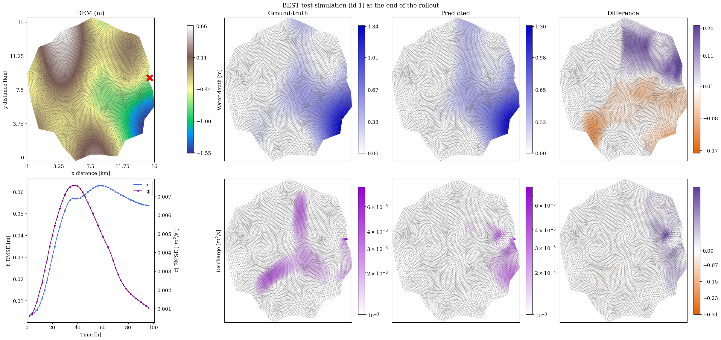
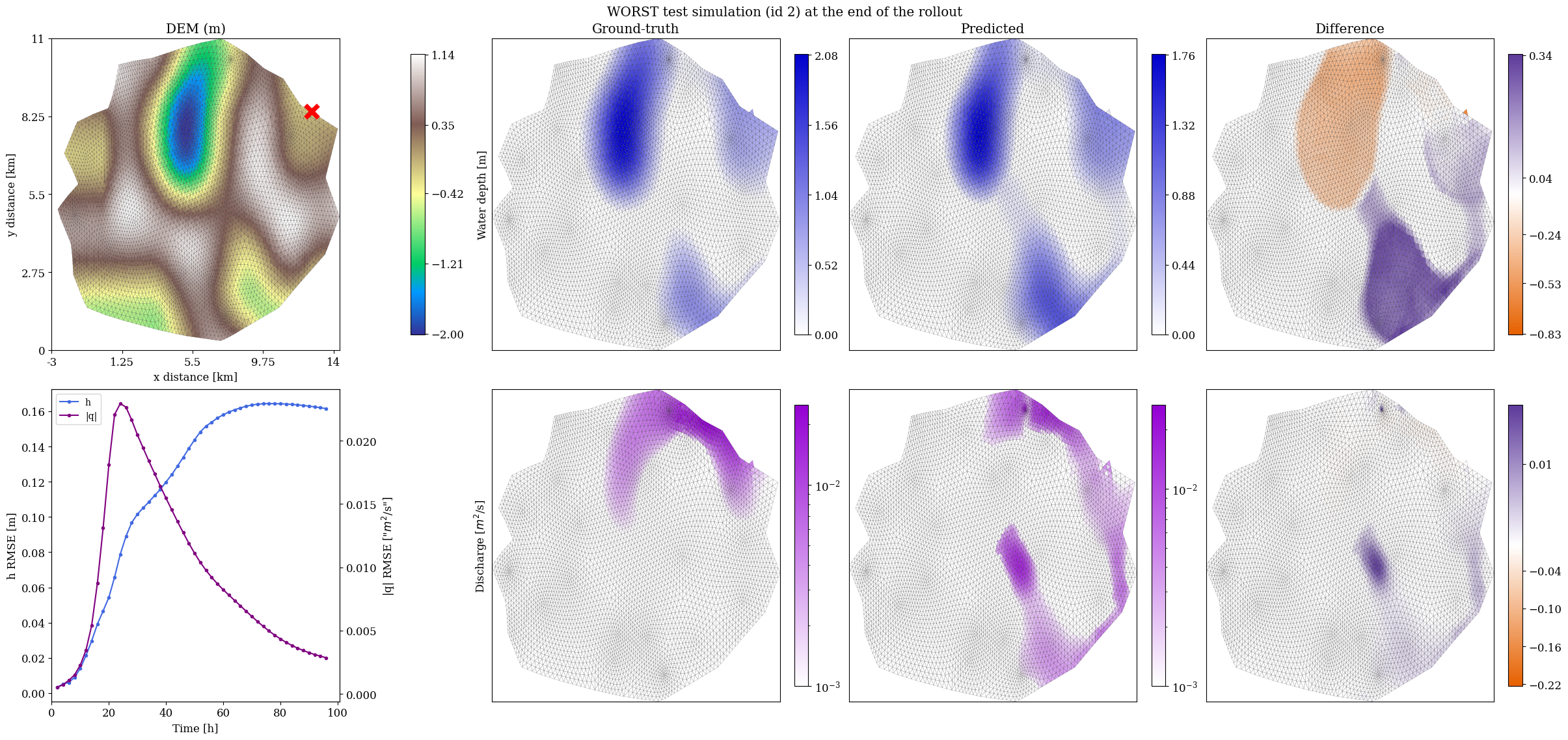
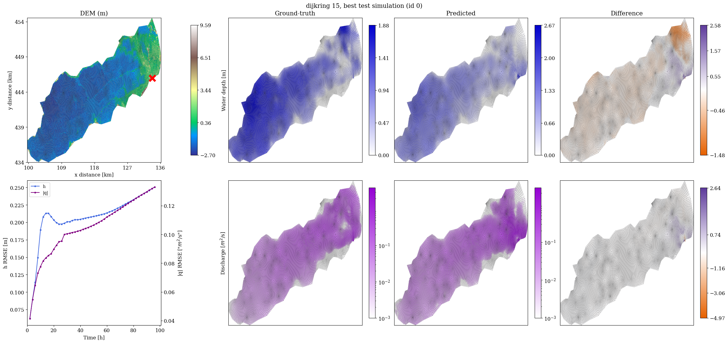
PlotRollout.explore_rollout is the authors' summary figure: DEM, ground-truth/predicted/error water-depth maps, discharge maps, and the error over time (scale=0 is the finest mesh). We look at the lowest-error simulation first, then the highest.

Water depth and discharge at selected times (best simulation)¶

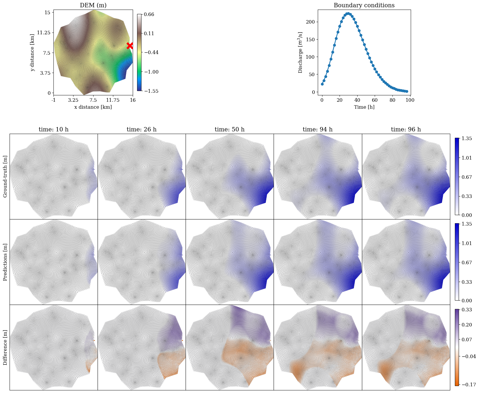
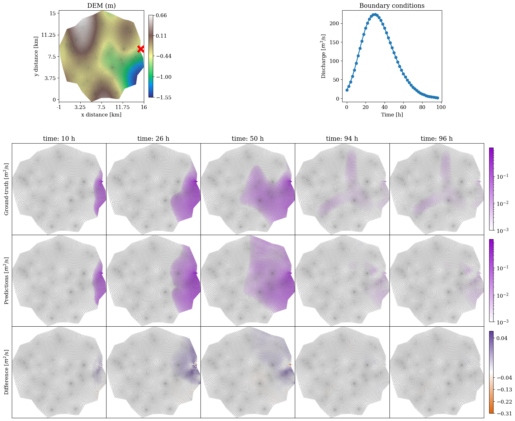
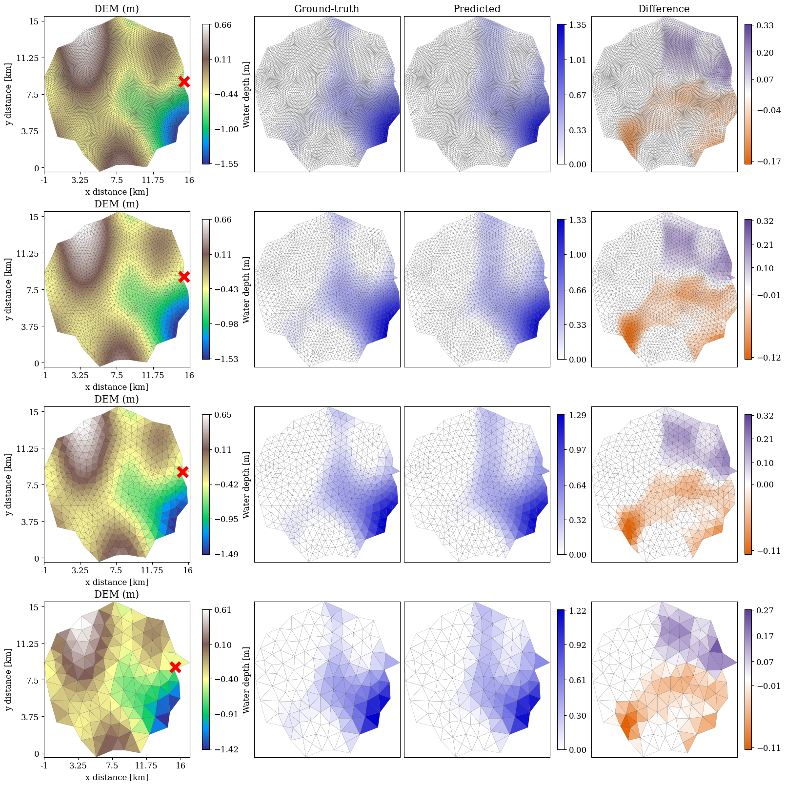
One row per time (8 h / 24 h / 48 h / 94 h): ground truth · prediction · difference.

The matching figure in the paper: unit-discharge rollout on the synthetic test set (Appendix A, paper Fig. 12)¶

Fig. 12 — $|q|$ for one synthetic test simulation on a logarithmic colour scale: ground truth (top), prediction (middle), difference (bottom). The model reproduces how the flood front advances into the domain and then recedes as the inflow weakens; the largest errors sit near the breach and along the path of the flood peak around 48 h, at a magnitude of 0.02 m² s⁻¹. The compare_v_rollout call above draws the same kind of figure.

Figure source: Bentivoglio et al., NHESS 25, 335–351, 2025, doi:10.5194/nhess-25-335-2025, CC BY 4.0.

Flood arrival time (FAT) and mass conservation¶

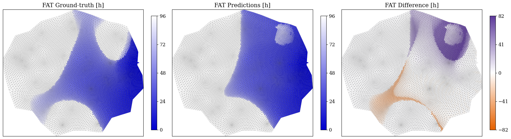
FAT is the time at which each cell first exceeds 0.05 m of water depth, one of the quantities emergency planners care about most. The mass-conservation plot compares the cumulative inflow volume with the water volume inside the domain.

The multi-scale view¶

Predicted water depth on all four scales at the same instant (the model also maintains a water field on the coarse scales, which is what carries information across scales).

4.1.5 Pareto front: speed versus accuracy (paper Fig. 7, Table A1)¶

Fig. 7 — mSWE-GNN (circles) and SWE-GNN (crosses) in the plane of speed-up against (a) validation RMSE and (b) validation CSI$_{0.05}$; colour is the parameter count and the dashed red line is each model's Pareto front. The key points:

• the mSWE-GNN Pareto front dominates SWE-GNN's — 2–4× faster at equal accuracy, and about 0.04 m lower RMSE at equal speed;
• the fastest mSWE-GNN variant exceeds a 1200× speed-up; it does not have fewer parameters than SWE-GNN, but it runs only 2–5 layers on the finest scale (the one with most nodes and edges) whereas SWE-GNN needs 10–18, and that is where the compute difference comes from;
• fewer layers also make training more stable (gap 2). The reference model selected in the paper is $L=4, G=64$, a compromise between speed and accuracy.

Table A1 — runtimes and speed-ups (the selected model)

Below we roll out each of the 16 checkpoints shipped with the repo and rebuild this Pareto figure (the paper uses the validation set, we use the test set).

Figure source: Bentivoglio et al., NHESS 25, 335–351, 2025, doi:10.5194/nhess-25-335-2025, CC BY 4.0.

In the code: reproducing the Pareto front over 16 checkpoints (K ∈ {2,3,4,5} × F ∈ {16,32,50,64})¶

The paper draws a Pareto front for a family of models in the speed-versus-accuracy plane. Here each checkpoint is rolled out again and plotted next to the values recorded in the repo. Set RUN_ALL_CHECKPOINTS=False to skip this (each model takes several minutes on CPU).

4.2 Transfer to the real case study: dike ring 15 (§4.2, paper Fig. 9–11, Table 2)¶

Applied directly to dike ring 15, a model trained only on the synthetic data reaches a CSI$_{0.05}$ of just 63 % (the hydrographs are out of distribution, see Fig. 6). After fine-tuning on a single simulation for about 20 min, the CSI$_{0.05}$ over the 10 test breaches rises to 87.68 % and the depth MAE falls from 0.31 m to 0.12 m.

Table 2 — effect of fine-tuning (10 test simulations, mean ± SD, finest mesh)

Fig. 9 — Water-depth rollout for one dike-ring-15 test breach (red cross, top left): ground truth (top), prediction (middle), difference (bottom). The model captures the overall dynamics of the flood spreading north-east across the low polder; the errors are mainly a systematic slight overestimate after 48 h (purple) and a local underestimate near the breach.

Fig. 10 — Flood arrival time for the same simulation (the moment each cell first exceeds 0.05 m). The predicted arrival-time field is nearly identical to the ground truth, with the differences concentrated at the tail of the flood front (±12–24 h). FAT is the quantity that matters most for evacuation planning.

Fig. 11 — CSI$_{0.05}$ of the fine-tuned model at all 10 test breach locations: 0.82–0.94, showing that fine-tuning on a single breach generalises to the rest of the ring, with different inflow directions and basin responses.

Figure source: Bentivoglio et al., NHESS 25, 335–351, 2025, doi:10.5194/nhess-25-335-2025, CC BY 4.0.

In the code: load finetuned_dk15.h5 and roll it out on the 10 dike-ring-15 test simulations¶

config_finetune.yaml fine-tunes on 1 dike-ring-15 simulation and tests on the remaining 10 (22 880 fine-mesh cells, about 30 000 nodes per sample). Here we only load the authors' fine-tuned checkpoint and test it.

4.3 Ablation study (§4.3, paper Table 3)¶

These numbers were transcribed from the article text; check them against the original table before quoting. The conclusion: the multi-scale module and the rotation-invariant inputs contribute most (removing either raises the test RMSE by about 17 %); the skip connections and the decoder form matter less but point the same way. This maps back onto the gaps in section 1: multi-scale addresses the range of propagation speeds and the instability of deep stacks, rotation invariance improves sample efficiency.

5. Discussion and conclusion (§5–6) + Appendix C¶

Strengths (against the four gaps of section 1)

1. The U-shaped multi-scale structure covers the domain with 2–5 layers per scale → it can represent fast and slow propagation, trains stably, and does little work on the finest scale → speed-ups of 700–1200× and a Pareto front that dominates SWE-GNN.
2. Ghost cells plus directed edges → a time-varying breach hydrograph can be used as an input.
3. Rolling out from a dry bed at $t=0$ → no numerical solver is needed for the initial condition.
4. Rotation-invariant inputs plus the graph structure → transfer to unseen meshes, topographies and boundary conditions, with a real case study needing only one simulation for fine-tuning.

Limitations (stated by the authors): only dike-breach floods were evaluated (not river, coastal or pluvial floods); time-varying water-level boundaries were not tested; roughness is spatially uniform; the mesh must be generated top-down from a boundary polygon, so an existing fine mesh cannot be used directly; multiple simultaneous boundary conditions were not considered; the number of layers is the same on every scale; and there is no comparison against newer methods such as Fourier neural operators or neural fields.

Future work: time-varying breach-growth models; adding water bodies and linear elements (roads, secondary dikes); precipitation input and coupling with 1-D drainage for urban flooding; probabilistic multi-scenario frameworks and uncertainty quantification; PINN-style auto-differentiation losses; larger training sets to remove the need for fine-tuning; JIT/IPU acceleration.

Appendix C: speed-up from parallel inference (paper Fig. 14)¶

Fig. 14 — Speed-up of the 16 Pareto models on the synthetic test set as a function of batch size, i.e. how many simulations are inferred in parallel (both axes log). Running 20 simulations in parallel buys another ~4.5×; models with more layers (larger dots) and more parameters (darker) benefit less. Counting the runtime of the one numerical simulation needed for fine-tuning, the overall speed-up on the real case study is about 4–8×.

Figure source: Bentivoglio et al., NHESS 25, 335–351, 2025, doi:10.5194/nhess-25-335-2025, CC BY 4.0.

In the code: the repo's recorded parallel-inference timings and mass-conservation experiment (read from csv, not re-run)¶

• batch_prediction_times.csv: inference time as a function of batch size (several simulations inferred in parallel).
• mass_conservation.csv: the effect of the mass-conservation loss weight (trainer_options.conservation) on accuracy.

6. Reproduction findings, and what the platform cost¶

Findings

• Training can be skipped entirely: the 17 checkpoints shipped with the repo are compatible with the current code and data, and test_model.py (or this notebook) is enough to test them.
• The published claims reproduce. Against the paper's abstract: water-depth MAE 0.05 m → 0.0510 m here; unit-discharge MAE 0.003 m² s⁻¹ → 0.0030; speed-up above 700× on the realistic case → 1187× on dike ring 15; CSI$_{0.05}$ 87.68 % after single-sample fine-tuning → 87.95 %. All four.
• A correction to an earlier version of this section. It reported that the depth error did not reproduce: RMSE 0.084 m against the 0.050 m in overview_MSGNN.csv. That comparison was wrong. The column named test roll loss WD in that csv holds an MAE, not an RMSE, despite its name and despite config.yaml setting type_loss: RMSE. The evidence, over all 16 checkpoints: our MAE differs from the recorded value by 0.0030 on average (ratio 1.00), our RMSE by 0.0367 (ratio 1.60) — and 1.60 is exactly our own RMSE/MAE ratio of 1.61. Per-model agreement reaches 0.0002. Sixteen independently trained models do not line up that way by chance. Comparing like with like, the depth error reproduces to about 2 %.
• What does still differ: flood extent, by about 3 % relative — CSI$_{0.05}$ 0.803 here against 0.830 recorded, CSI$_{0.3}$ 0.658 against 0.687. The likeliest cause is that the pickles were rebuilt with meshkernel 3.0.0, so the coarse meshes may differ slightly from the authors'. Not verified.
• The general lesson, twice over in this one reproduction: check what a number is before comparing it. The first mix-up (test_model.py prints MAE while main.py logs RMSE) was caught early; the second survived longer because the config said RMSE and that was believed instead of tested against the values themselves.

Pitfalls, and which machine each one belongs to

This was reproduced on two unrelated systems: an HPC cluster with H100 nodes, and the I-GUIDE Platform's CPU JupyterHub. Items 1, 2 and 8 are properties of the code and will follow you anywhere. Items 3 to 6 are the I-GUIDE hub. Item 7 was the cluster only, and is recorded because it shows how much of "reproduction difficulty" is really local infrastructure.

1. lightning must be exactly 2.0.9.post0 (see requirements.txt). Version 2.1 and later raise a TypeError because plmodule.load_from_checkpoint is called on an instance.
2. Lightning ≥2's WandbLogger is lazy. Calling fix_dict_in_config straight after constructing it raises You must call wandb.init() before wandb.config.keys. This notebook calls wandb.init(mode="disabled") first.
3. The container is capped at 8 GiB. conda env create gets OOM-killed while parsing conda-forge repodata and prints only Killed. Build the environment with python -m venv and pip instead. Disk is not the constraint: home is measured in terabytes.
4. unzip is not installed. Python's zipfile module substitutes.
5. None of the ~26 preinstalled kernels is usable. geoai is the closest — PyTorch 2.4.0, no torch_geometric — and none of them carries the required lightning pin.
6. Zenodo intermittently answers 502/504 on the dike-ring-15 archive. wget -c resumes.
7. On the HPC cluster, Zenodo's API and web pages returned 403 while direct file URLs worked, and the system curl was broken. Neither problem appeared on I-GUIDE.
8. The archive ships lower-case polygon_{i}.pol while create_mesh_dataset opened Polygon_{i}.pol. One word changed at database/graph_creation.py:1612 — the only edit made to upstream code in this whole reproduction; the original is kept alongside it.
9. For a full training run (200 epochs) use sbatch scripts/sbatch_gpu_real.sh with max_epochs set back to 200.